I just enrolled in Coursera’s Machine Learning course taught by Andrew Ng. The class doesn’t start until the 30th but they have released the first week’s material. In this post I will go over the general concepts that I have cover so far.
Supervised Machine Learning
The most important difference is that supervised learning is given data to learn from where unsupervised learning is left to learn on its own. There are two types of problems we learned about, regression and discrete.
Regression
Supervised learning is an algorithm that is taught with the right answers from the start. For example, if we were given housing data that contained prices and square footage we would use that data to train our algorithm.
This is considered a regression problem because we are trying to fit the algorithm to a continuous value - housing price. This differs from discrete because we don’t have clear boundaries in the answer. Regression problems can be modeled in many different ways. We could use a linear regression, quadratic, or many other modeling techniques.
Discrete
Discrete learning problems are also taught but they tackle a different type of data. The housing price example was a regression problem but if we changed the question to “Will this house get sold?”, this would be a discrete problem. The difference being that sold is a discrete value. It is either sold or it isn’t. Housing prices can be an number making the possibilities much more vast.
An example from the course was using tumor size and age of a patient to predict whether the tumor is malignant or benign. Malignant or benign is either or. There is no scale between the two.
Unsupervised Machine Learning
Unsupervised means the algorithm takes the data and tries to make sense of it. We don’t give it correct answers to train it.
Examples of Unsupervised Machine Learning
- Social networks determining who you are friends with and what you will find interesting
- Market segmentations from a group of customers. Which customers are similar
- Google news grouping like news stories together
These are examples of clustering. An unsupervised algorithm takes data and groups it into meaningful clusters.
Linear Regression with One Variable (Univariate)
This takes one input and predicts what the output should be. This is modeled using a single variable in a hypothesis function.
Here is an example hypothesis function that I worked with:
Let’s try to apply our hypothesis function to this data below.
| input($x$) | output($h_\theta(x)$) |
|---|---|
| 0 | 4 |
| 1 | 7 |
| 2 | 7 |
| 3 | 8 |
We start by choosing values for $\theta_0$ and $\theta_1$ and calculate how well they model our data. For this examples we will use and . Our new hypothesis function is:
Using our input values lets sum outputs and compare them to our actual outputs.
If we add up the output column we get 26 which is 6 off. This is called the cost. The goal of a linear regression is to minimize cost.
The Cost Function
This function iterates over each row in a dataset and applies our hypothesis function to it and compares it to our expected value. The in the sum corresponds to a row and is the number of rows. Using our table above, it would apply to each input value and compare it to the output. It returns an average of how wrong we were for our guess.
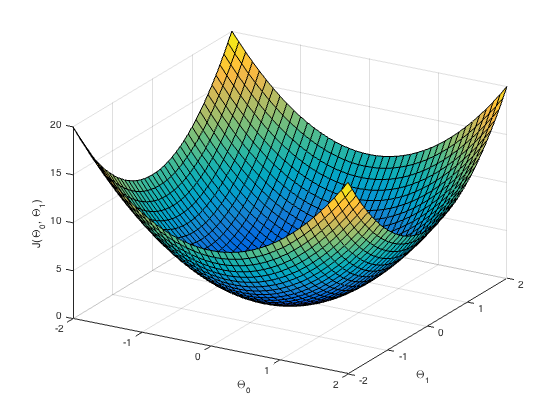
Using , , and we can plot a point that represents the cost for those two values. We can create a graph from the points and find our local and absolute minimums to find the lowest possible cost. With these values we have found our most accurate values.

In the plot above our ideal values for and are where is at a minimum.
In my next post I will write about Gradient Descent, which is a way to traverse Cost plots to find the minimum.